Following on from the previous post, in this post we will be outlining our initial work on using cameras and machine vision to quantify print performance – measuring the width of printed tracks in different conditions. Future blogs will discuss how we are applying this to various problems.

Track Width Measuring System Overview

Measuring the width of a FDM deposited track is conceptually quite simple. We produce gcode describing a path, print it, and then perform an imaging pass along the same path with a tool mounted camera. We then take the images and measure the width of the line in pixels

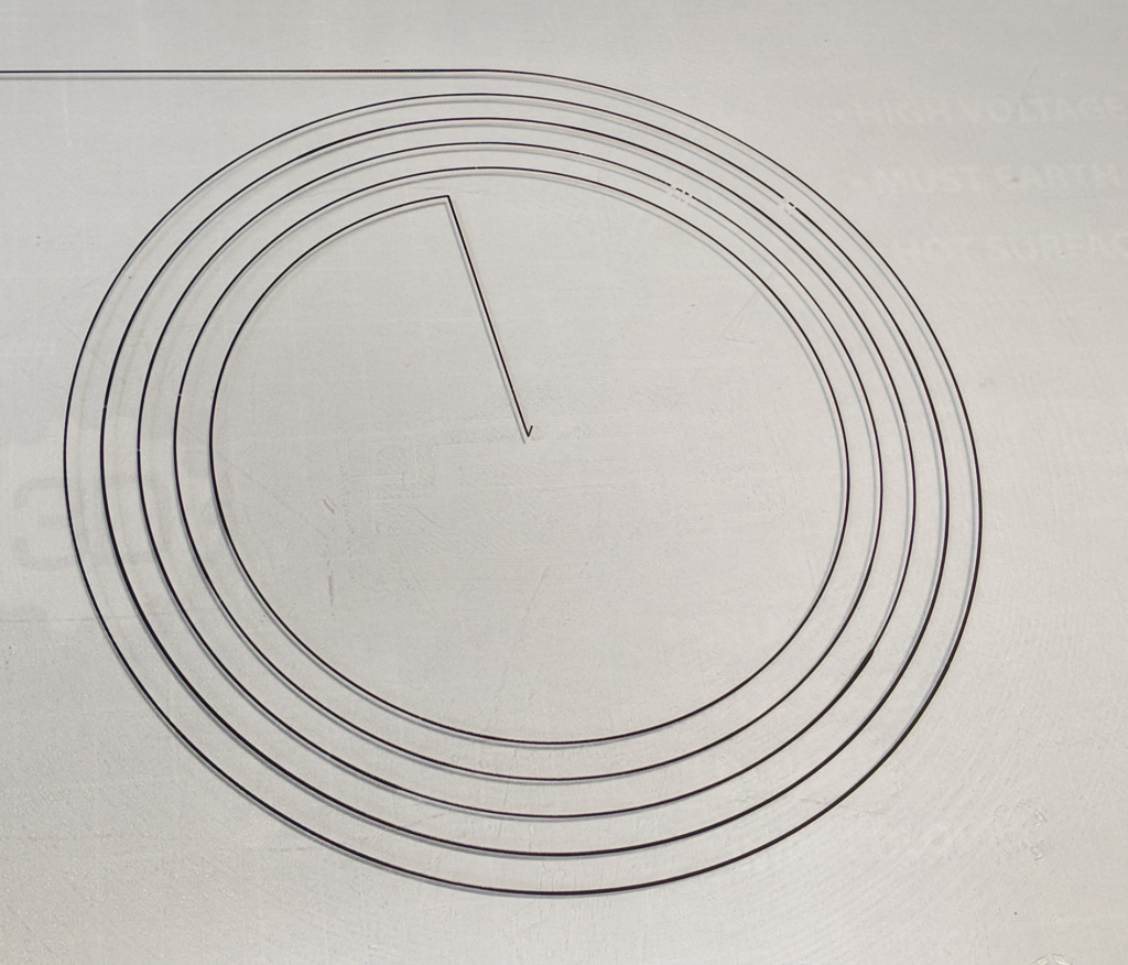Image of a spiral track printed with varying line width ready for imaging.

The pixel width can be converted into units of distance by calibrating the camera and measuring something of known width, however, this latter step has been unnecessary for our applications.

Video showing the imaging of a printed track with the measurement overlaid as a visualisation.

For our initial work we have used a low cost USB microscope (called an “endoscope” by the online retailer), mounted to a E3D toolchanger as a tool.

USB microscope mounted on an E3D toolchanger

This allows us to switch between a print tool and imaging tool. It would be quite possible to mount the camera on the printing head (as we did with the raspberry pi camera in the previous imaging system covered in our post about initial work on defect detection, but the toolchanger system means that we can experiment with a range of cameras quickly, adjust the working distance of the camera in software without worrying about collisions with the nozzle or a restricted print volume.

The camera is attached to a Raspberry Pi SBC, which is connected to the Duet 3 controller over the SPI bus. The Raspberry Pi does the image processing that calculates the width and angle of the printed track, and combines it with data on machine position obtained from the Duet using the Duet Software Framework API. This is written to a file and analysed externally.

Complications

There are two complicating issues that must be considered for the imaging system to function correctly:

1. The latency of the image acquisition and processing. When using a USB camera with a low data rate and a relatively lower powered SBC for processing it is important to consider the time required to transfer the data and process it. As Raspberry Pis are prone to heat throttling during intensive use, the latency can be somewhat variable. The calculation of the line width itself is not particularly intensive, but copying the image data across memory and displaying user feedback is. The effect latency can be completely removed by bringing the camera to a complete stop, and waiting for the imaging to take place. This is useful for verifying the absence of latency artefacts, but makes the imaging step very slow.
2. The latency and granularity of the machine position reported by the Duet controller. The Duet does not report the exact machine position at the time of the request, but the end position of the current segment. (Note in RRF 3.3 Stable there is an option to segment moves to avoid this issue by setting a segment shorter than the distance between each image)

The strategy we employ, therefore, is to segment the imaging gcode into small (e.g. 0.5mm segments) move the camera at a constant velocity at a speed such that at least two images are taken per segment on average. During post processing we account for greater or fewer images.

The imaging location, therefore, is typically accurate up to the resolution of the segments.

Image Processing and Line Widths

The software for calculating the line widths from images has been written with the possibility of porting to a separate microcontroller in mind, as such it is optimised for the very specific task of measuring line width and angle.

Currently, the process of calculating track width is as follows:

1. Estimate width and angle based on where it crosses horizontal lines a. Pick “n” locations along either side of the image. b. For each location, starting with the outside examine each pixel inwards until a threshold condition is met, this provides a list of points along the edge of the track. c. Reject any points that don’t lie within a central region. d. Fit a line to the points. e. If fit is “good enough” (low residual variance, sufficient number of points) on both sides we use them in step 3, if not, we don’t use this data at all.
2. Repeat 1 but with vertical lines
3. Gather a consensus based on lines from 1 and 2, and calculate an initial track width and track direction
4. Refine the estimate by examining points on lines perpendicular to the track direction

1c and and 1e are typically sufficient to remove minor artefacts such as small particles on the print bed. The consensus found in step 3 is typically very good, and perfectly good for most applications, however, there are certain directions (at 45 degrees) with a small systematic bias that becomes apparent with tracks of changing thickness. This motivates step 4, which removes this bias to all practical extent.

Test Patterns

Now that we have a reliable system for measuring the output from an extruder in terms of line width at a specific point on a print we can look at running a series of input test patterns through the system. This will allow us to characterise the extrusion system. The next few blog posts will go into detail on the various methods we used however, as a start point here is one example of using a step function of feed rate from 10 to 30mm/s and an expected output from a bowden extrusion system, with the elasticity of the bowden system taken into account. the predicted line width (in arbitrary units) is shown in the third graph.

Step response from 10-30mm/s input, the expected output of the extruder and the forecast effect on line width