Making reliable measurements of the extrusion system requires a controllable and repeatable system. Ideally, to measure the width of extruded filament we would print a long straight continuous line over a perfectly flat surface. This ideal, however, is impossible with the constraints of a standard 3D printer. At some point you need to stop or change direction, and doing this affects the processes that determine the output of the printer. The kinds of effect that pressure advance corrects for take place over a period of seconds or tens of seconds, making the bed size a problematic constraint!

To get as close as possible to this ideal with our printers, we have been using a spiral shaped path. This allows us to look at the print performance with different speeds and feeds, without being forced to make any radical changes in direction. This is not perfect, but is close enough to get some useful data. We’ve shown an image of this kind of test before, but here it is again:

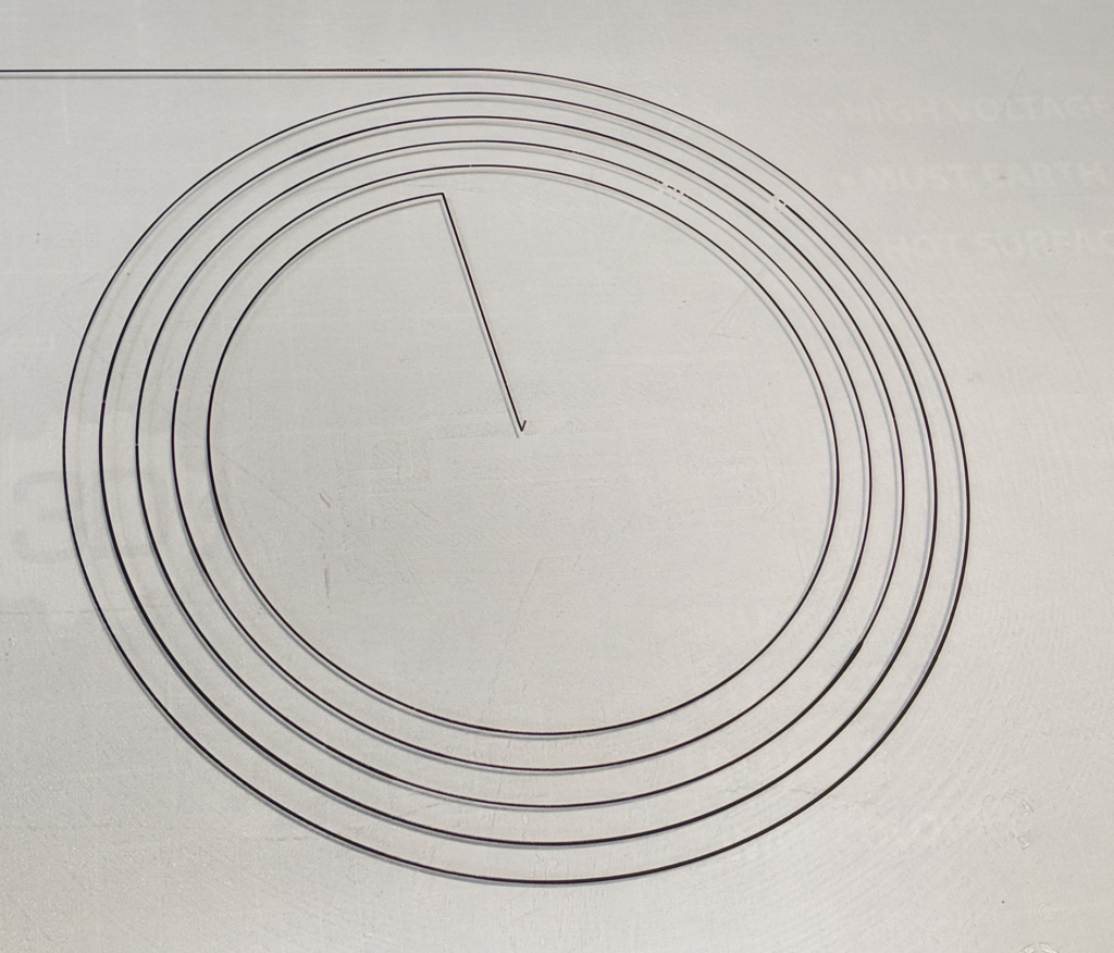Image of a spiral track printed with varying line width ready for imaging.

Systemic challenges

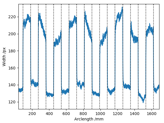
Below is a plot of the measured width of two spiral paths with a nominally constant width and print speed. Underneath is the angle around the centre point. We can see that there is a change in width with the position (or perhaps direction) of the print.

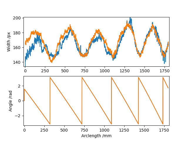Image showing the periodicity of variation is the measured width of a constant speed spiral varied based on the angle along the spiral.

Additionally, there are a number of smaller, higher frequency, artefacts present that can be exploited to extract details about the extrusion process. These artefacts can be seen in the plots below.

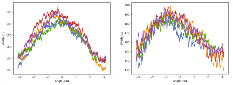Measurement of printed track width for a commanded constant width spiral at two different speeds. Each trace within a figure is a 360 degree section of the spiral. The high frequency oscillations within the traces change with speed, their analysis will be in a future post.

In later blog posts we will go into why both the large oscillations in overall line width around the bed are happening (spoiler: it’s not because the bed is not level) and also some of the causes of the high frequency artefacts.

Calculating Pressure Advance Parameters From Step Changes

In our last post we showed the theoretical effect of the Bowden on track width when the feed rate is stepped up or down. Now it is time to measure it.

The tests we will show here involve moving the nozzle at constant speed, whilst varying the commanded output in a stepwise fashion. This will give a width that is proportional to the rate that filament extruded, and a position along the spiral that is proportional to time. It is a bit easier to analyse this setup than one where the bed speed and extrusion speed are kept proportional (i.e. constant commanded width).

In these tests we switch between printing slowly and printing fast at regular time intervals . These are not synchronised with the angle around the centre, so we can “wash out” any changes due to the position like the periodic artefacts shown before by averaging over the entire print.

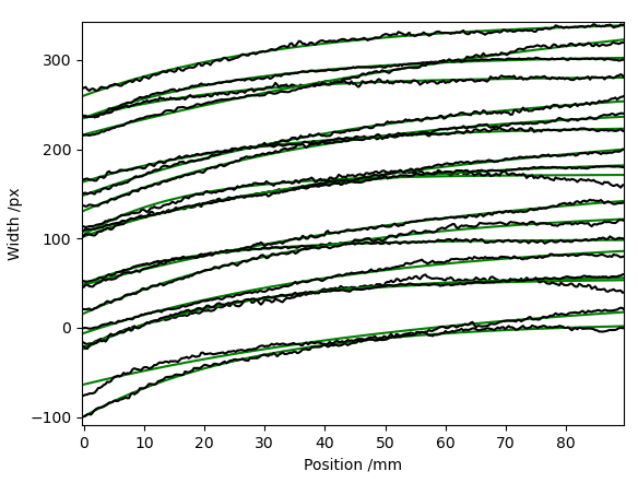
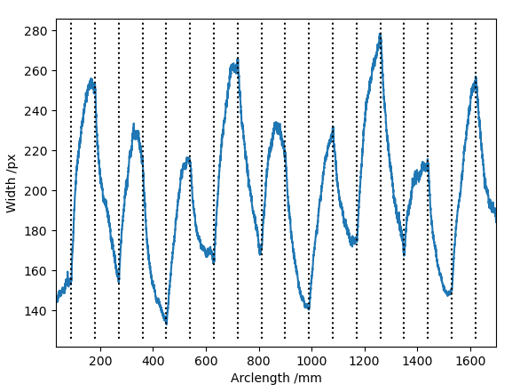Example output of a test print with a slow exponential decay caused by an approximately 60cm Bowden. The decay has a half-life of about 6 seconds, which corresponds to a pressure advance constant of about 4.2 (6*log(2)).

You might notice that the x-axis is in mm rather than units of time. As the processes in the Bowden depend (primarily) on time, running the print at different speeds gives different decay constants when measured in terms of position.

This provides a good way of making sure our results are robust: We can run prints with different spatial frequencies, causing the step changes to occur at different points along the spiral and providing a way of checking against errors induced by any speed dependent noise sources.

Extracting the Pressure Advance Constant

Calculating the pressure advance constant is just a matter of fitting an exponential curve to this data. We take the data above and split it into sections, and flip every other one upside down to make them comparable.

We can then fit the data with a exponential function of the form:

Where A, B and C are found by the fitting algorithm. We don’t really care about the values of A and B, but they need to be there to fit properly. We only need the value of the exponent C, as that is related to the pressure advance constant.

Above we show it applied to the individual sections. However, it is better to average the signals before calculating the exponent. This is important because the exponent calculation can be very sensitive to the periodic offset shown in the first diagram above, and averaging these estimated exponents can give a biassed value.

The constant C from the fit will be in units of mm¯¹ to convert it to the pressure advance constant ∝ which is defined in units of seconds. The conversion is as follows:

Where R is the movement speed along the bed in mm/s, i.e. 60 times the “F” parameter in the gcode.

Direct Drive Comparison

Running the same test on a print using a direct drive extruder gives much sharper transitions.

Example output of a test print showing the slow exponential decay in a direct drive extruder. The decay has a half-life of about 0.06 seconds, which corresponds to a pressure advance constant of about 0.041 (0.06log(2)).Example output of a test print showing the slow exponential decay in a direct drive extruder. The decay has a half-life of about 0.06 seconds, which corresponds to a pressure advance constant of about 0.041 (0.06log(2)).

This seems to work and give reasonable results. The measured pressure advance constant was 100 times shorter. It seems to work and give reasonable results on direct drive, unlike the figure of 4.2 for bowden which is higher than often used.

Comparison with a Standard Pressure Advance Calibration Print

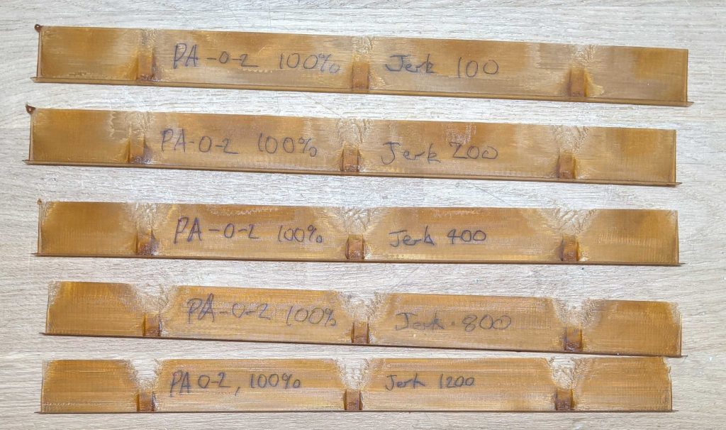Examples of test prints varying PA constant from 0-2 and extruder jerk from 100-1200 as shown with transparent PLA at manufacturer temperatures.

Examples of test prints with transparent PLA at manufacturer temperatures, results for the pressure advance constant

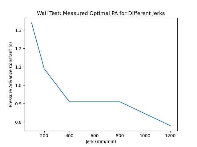
This is an unexpectedly large variation in PA constant based on extruder jerk. In the next post(s) we will explore this, along with the difference in the measured pressure advance constant from the spiral tests and the print tests.